Statistical Data Analysis – Statistics Assignment Sample
Assignment
On
Data Analysis
Submitted To
Submitted By
Task 1 1. Descriptive statistics
The descriptive statistics showing mean, median, mode, standard deviation, variance and range for the start-up costs of the five businesses as provided in the given data are shown as below:
| Table :1 Descriptive Statistics | |||||
| Pizza (X1) | Baker (X2) | Shoe-store (X3) | Gift Shop (X4) | Pet Store (X5) | |
| Mean | 83.00 | 92.09 | 72.30 | 87.00 | 51.63 |
| Median | 80 | 87 | 70 | 97.5 | 49 |
| Mode | 35 | Nil | Nil | 100 | 30 |
| Standard Deviation | 34.13 | 38.89 | 31.37 | 35.90 | 27.07 |
| Sample Variance | 1165.17 | 1512.69 | 983.79 | 1289.11 | 733.05 |
| Range | 105 | 120 | 90 | 115 | 90 |
2. Frequency distribution and histogram
(a) Frequency and relative frequency distribution of various businesses
(i) Frequency distribution of business X1 (Pizza)
| Bin | Class Interval | Frequency | Relative Frequency |
| 30 | 0-30 | 0 | 0.0 |
| 60 | 30-60 | 4 | 0.333 |
| 90 | 60-90 | 3 | 0.250 |
| 120 | 90-120 | 3 | 0.250 |
| 150 | 120-150 | 2 | 0.167 |
| Total | 12 | 1.0 |
(ii) Frequency distribution of business X2 (Baker)
| Bin | Class Interval | Frequency | Relative Frequency |
| 30 | 0-30 | 0 | 0.0 |
| 60 | 30-60 | 3 | 0.27 |
| 90 | 60-90 | 4 | 0.36 |
| 120 | 90-120 | 2 | 0.18 |
| 150 | 120-150 | 1 | 0.09 |
| 180 | 150-180 | 1 | 0.09 |
| 11 | 1 |
(iii) Frequency distribution of business X3 (Shoe store)
| Bin | Class Interval | Frequency | Relative Frequency |
| 30 | 0-30 | 0 | 0 |
| 60 | 30-60 | 4 | 0.4 |
| 90 | 60-90 | 3 | 0.3 |
| 120 | 90-120 | 2 | 0.2 |
| 150 | 120-150 | 1 | 0.1 |
| 10 | 1 |
(iv) Frequency distribution of business X4 (gift shop)
| Bin | Class Interval | Frequency | Relative Frequency |
| 30 | 0-30 | 0 | 0 |
| 60 | 30-60 | 3 | 0.3 |
| 90 | 60-90 | 1 | 0.1 |
| 120 | 90-120 | 5 | 0.5 |
| 150 | 120-150 | 1 | 0.1 |
| 10 | 1 |
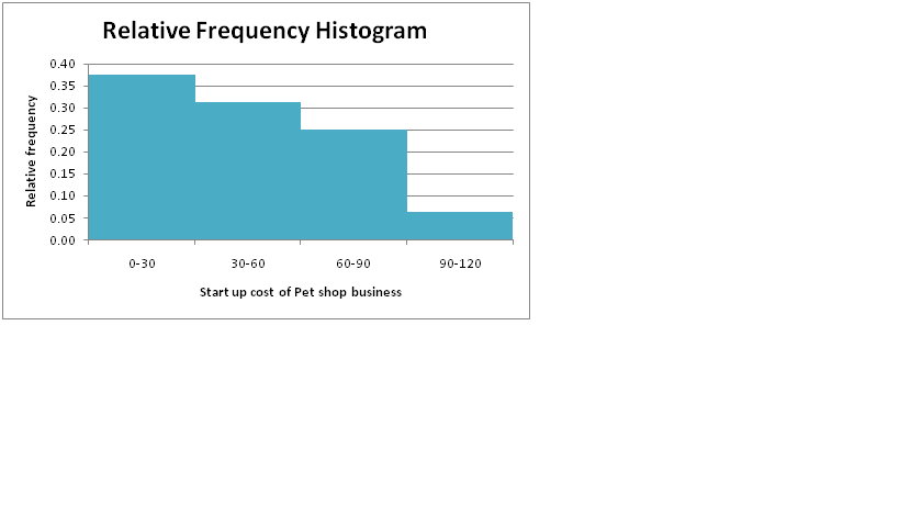
(v) Frequency distribution of business X5 (Pet store)
| Bin | Class Interval | Frequency | Relative Frequency |
| 30 | 0-30 | 6 | 0.38 |
| 60 | 30-60 | 5 | 0.31 |
| 90 | 60-90 | 4 | 0.25 |
| 120 | 90-120 | 1 | 0.06 |
| 16 | 1.00 |
(b) Relative frequency histogram
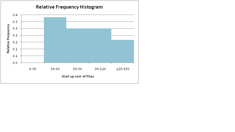
(i) Relative frequency histogram of business X1 (Pizza)
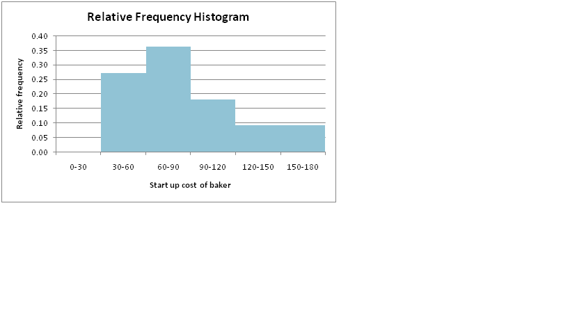
(ii) Relative frequency histogram of business X2 (Baker)
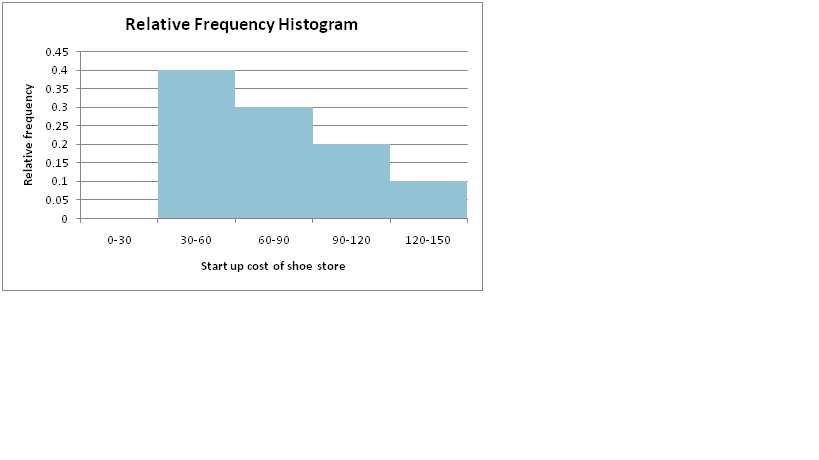
(iii) Relative frequency histogram of business X3 (Shoe store)
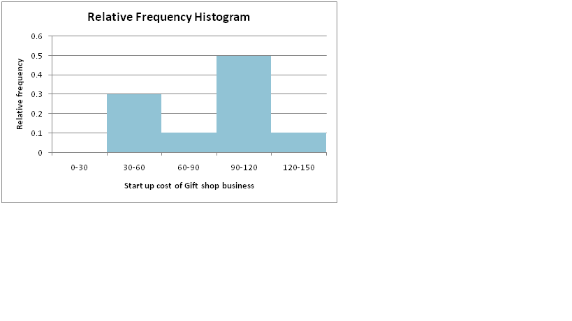
(iv) Relative frequency histogram of business X4 (gift shop)
(v) Relative frequency histogram of business X5 (Pet store)
3. Discussion on results of descriptive statistics and histograms Descriptive statistics
- Mean of the start-up cost of various businesses represent the average value of cost. It is 51.63 in case of pet shop which is the lowest value and highest in case of baker business which is 92.09.
- Median is the middle value of the start-up costs. It is 49 in case of pet shop business which is lowest value and 97.5 in case of gift shop which is the highest value.
- Mode depicts the cost which is happening most number of times. Pet store business has lowest mode value which is 30 and gift store has highest mode which is 100.
- Standard deviation of cost shows the risk of variation of cost from the average cost. Pet business has the lowest standard deviation which implies that the level of risk is low in this business. The bakery business has standard deviation of 38.89 which is the highest value. It means this business has high risk level.
- Variance is also a representative of risk factor as it is the square value of standard deviation. The business with highest variance has highest risk level.
- Range depicts the difference largest and smallest value. Pet business has lowest range of 890 and bakery business has highest range of 120.
Overall the analysis depicts that the investment required for pet business is low and it has lowest risk as well.
Frequency and relative frequency distribution and histograms
The frequency distribution shows the number of times the costs lie within a class interval. The relative frequency distribution shows the frequency in relative terms with respect to total frequency.
(i) In case of pizza business, costs lying within the range of 0-30 are nil. Maximum costs lie within the range of 30-60 and least costs lie within the range of 120-150.
(ii) In case of baker business, costs lying within the range of 0-30 are nil. Maximum costs lie within the range of 60-90 and least costs lie within the range of 120-150 and 150-180.
(iii) In case of shoe-store business, costs lying within the range of 0-30 are nil. Maximum costs lie within the range of 30-60 and least costs lie within the range of 120-150.
(iv) In case of gift shop business, costs lying within the range of 0-30 are nil. Maximum costs lie within the range of 90-120 and least costs lie within the range of 60-90 and120-150.
(v) In case of pet store business, maximum costs lie within the range of 0-30 and least costs lie within the range of 90-120.
4. Test of significance (ANOVA)
The significance of difference in start-up costs of various costs has been tested with the help of ANOVA.
(a) Hypothesis
H0: µ1 = µ2 = µ3 =µ4 = µ5
There is no significant difference in the mean startup cost of given five businesses.
H1: µ1 ≠ µ2 ≠ µ3≠ µ4 ≠ µ5
There is significant difference in the mean startup cost of given five businesses.Where
µ1 shows the average start-up cost of pizza business
µ2 shows the average start-up cost of baker business
µ3 shows the average start-up cost of shoe store business
µ4 shows the average start-up cost of gift shop business
µ5 shows the average start-up cost of pet shop business
The excel output is given as below:
SUMMARY
| Groups | Count | Sum | Average | Variance |
| X1 | 13 | 1079 | 83 | 1165.167 |
| X2 | 11 | 1013 | 92.09091 | 1512.691 |
| X3 | 10 | 723 | 72.3 | 983.7889 |
| X4 | 10 | 870 | 87 | 1289.111 |
| X5 | 16 | 826 | 51.625 | 733.05 |
ANOVA
| Source of Variation | SS | df | MS | F | P-value | F critical |
| Between Groups | 14298.22424 | 4 | 3574.556 | 3.246336 | 0.018391 | 2.539689 |
| Within Groups | 60560.75909 | 55 | 1101.105 | |||
| Total | 74858.98333 | 59 |
The null hypothesis is rejected as the p-value is 0.018 which is less than 0.05. It means there is there is significant difference in the mean startup cost of given five businesses.
Task 2
For All Greens Pty Ltd. six variables are given out of which sales is the dependent variable and rest all are independent variable.
(i) Excel output and estimated regression equation:
The excel output of multiple regression model is shown as below:
SUMMARY OUTPUT
| Regression Statistics | |
| Multiple R | 0.9966 |
| R Square | 0.9932 |
| Adjusted R Square | 0.9916 |
| Standard Error | 17.6492 |
| Observations | 27 |
ANOVA
| df | SS | MS | F | Significance F | |
| Regression | 5 | 952538.9 | 190507.8 | 611.5903672 | 5.39731E-22 |
| Residual | 21 | 6541.4 | 311.5 | ||
| Total | 26 | 959080.35 |
| Coefficients | Standard Error | t Stat | P-value | Lower 95% | Upper 95% | Lower 95.0% | Upper 95.0% | |
| Intercept | -18.859 | 30.150 | -0.626 | 0.538 | -81.560 | 43.841 | -81.560 | 43.841 |
| X2 | 16.202 | 3.544 | 4.571 | 0.000 | 8.831 | 23.573 | 8.831 | 23.573 |
| X3 | 0.175 | 0.058 | 3.032 | 0.006 | 0.055 | 0.294 | 0.055 | 0.294 |
| X4 | 11.526 | 2.532 | 4.552 | 0.000 | 6.260 | 16.792 | 6.260 | 16.792 |
| X5 | 13.580 | 1.770 | 7.671 | 0.000 | 9.898 | 17.262 | 9.898 | 17.262 |
| X6 | -5.311 | 1.705 | -3.114 | 0.005 | -8.858 | -1.764 | -8.858 | -1.764 |
The regression equation of sales on five independent variables is as follows
Y = -18.86+ 16.20*X2 + 0.18*X3 + 11.53 X4+ 13.58 X5-5.31X6
Where Y= Annual net sales, X2= area, X3 = inventory, X4 = advertisement expense, X5 = size of sales districts, X6 = Number of competing stores
(ii) Fitness of the regression equation
The value if R-square indicates the goodness of fit of a model. The model is deemed to be fit if he value of R-square lies within the range of 70% to 100%. The value of R-square in the model is 0.99. It means that model is good as the 99% of the changes in sales are because of the independent variables considered.
(iii) Test of significance
H0: There is no significant relationship between sales and other given variables.
H1: There is significant relationship between sales and other given variables.
The null hypothesis is rejected as the p-value is 0 which is less than 0.05. It means there is there is significant relationship between sales and other given variables.
(iv) Interpretation of slope coefficient
The slope coefficient shows that with a unit change in independent variable, how much change takes place in dependent variable.
(a) The slope coefficient of area is 16. It means for every unit change in area, the change in sales will be equal to 16.
(b) The slope coefficient of inventory is 0.17. It means for every unit change in inventory, the change in sales will be equal to 0.17.
(c) The slope coefficient of advertisement is 11.53. It means for every unit change in advertisement, the change in sales will be equal to 11.53
(d) The slope coefficient of sales district’s size is 13.58. It means for every unit change in size, the change in sales will be equal to 11.53 times
(e) The slope coefficient of number of competing stores is -5.3. It means for every unit increase in number of competing stores, the decline in sales will be equal to 5.3 times.
(v) Confidence intervals at 95%
The lowest and highest limits of intervals are given as below:
| Coefficient | TINV( 0.05,23) | SE | TINV( 0.05,23) *SE | Lower Limit | Higher Limit | |
| X2 | 16.20 | 2.07 | 3.54 | 7.33 | 8.87 | 23.53 |
| X3 | 0.17 | 2.07 | 0.06 | 0.12 | 0.06 | 0.29 |
| X4 | 11.53 | 2.07 | 2.53 | 5.24 | 6.29 | 16.76 |
| X5 | 13.58 | 2.07 | 1.77 | 3.66 | 9.92 | 17.24 |
| X6 | -5.31 | 2.07 | 1.71 | 3.53 | -8.84 | -1.78 |
(vi) Test of significance level of slope coefficient
| Variable | p-value | Interpretation |
| Area (Square feet) | 0 | P-value is less than 0.05. It means the slope of area is significant. |
| Inventory | 0 | P-value is less than 0.05. It means the slope of inventory is significant. |
| Advertisement expense | 0.006 | P-value is less than 0.05. It means the slope of advertisement expense is significant. |
| Size of sales district | 0 | P-value is less than 0.05. It means the slope of size of sales district is significant. |
| Number of competing stores | 0.005 | P-value is less than 0.05. It means the slope of competing is significant. |
(vii) No insignificant variable
All variables are significant as the p-value of all independent variable is less than 0.05. It means there is no insignificant variable which needs to be deleted. The regression equation as determined earlier will remain same.
(viii) Estimation of sales
Sales are to be estimated for a franchisee which has 1,000 sq ft floor area, $150,000 inventory, $5,000 spent on advertising, 5,000 families in the area of operation and 2 competitors.
Y = -18.86+ 16.20*X2 + 0.18*X3 + 11.53 X4+ 13.58 X5-5.31X6
Y = -18.86+ 16.20*(1) + 0.18*(150) + 11.53(5) + 13.58(5)-5.31(2)
= -18.86+16.20+27+57.65+67.9-10.62
= 139.27
References
Laerd Statistic. (2014). One-way ANOVA. Retrieved May 2017, from https://statistics.laerd.com: https://statistics.laerd.com/statistical-guides/one-way-anova-statistical-guide.php
Laerd Statistics. (2013). Descriptive and Inferential Statistics. Retrieved from https://statistics.laerd.com: https://statistics.laerd.com/statistical-guides/descriptive-inferential-statistics.php
Statistica. (2015). http://www.statsoft.com. Retrieved May 2017, from http://www.statsoft.com/Textbook/Multiple-Regression
Statistics Solutions. (2014). What is Multiple Linear Regression? Retrieved May 2017, from https://www.statisticssolutions.com/what-is-multiple-linear-regression/